gsopt

GSOpt: Human-in-the-loop Batched Optimization

Contents

1. Overview
2. Google Sheet Usage
3. Backend Architecture
4. The Optimizer
5. Pros and Cons
6. Recommendations and Examples
7. Benchmark Test Results

---

Find the latest version here.

Overview

Optimizing real-world engineering problems is often challenging. When the function you want to optimize is expensive, noisy, and lacks a simple mathematical form (aka “black box”, with no information on the derivatives of the function), many traditional methods fall short. GSOpt is designed for this type of problem by implementing a human-in-the-loop batched submission optimization workflow for noisy black box problems. The optimization process is orchestrated through a Google Sheet, so it’s easy to use for engineers.

The basic workflow is:

1. The optimizer suggests a batch of initial points based on the parameter settings.
2. You run the experiments and copy the results into the Google Sheet.
3. Ask the optimizer for new promising points, and use the analysis plots to keep track of the optimization. Repeat as necessary.

The Google Sheet acts as the central hub, storing all experimental data, providing basic analysis plots, and serving as the user interface for interacting with the optimization engine. All the optimization code and macros are in this repo: https://github.com/PaulENorman/gsopt.

Google Sheet Usage

Make a Copy of the Sheet

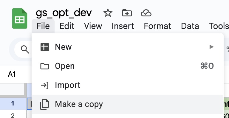
To use GSOpt, first save a copy of the template to your own Google Drive:

• Open the template sheet, then go to File → Make a copy.
• Save it to your Drive. Your copy will have its own bound Apps Script project.

Opening the Sidebar

To begin, click Extensions → GSOpt → Open Sidebar from the top menu to open the optimization sidebar.

Sheet Tabs Overview

The workbook contains three main tabs:

• Data: Where you enter your experimental results and view all optimization runs.
• Analysis: In-sheet charts showing progress and parameter relationships. Charts update automatically when objective values are edited.
• Parameter Settings: Configure your optimization parameters (names, bounds, objective name, etc.).

Optimizer Settings

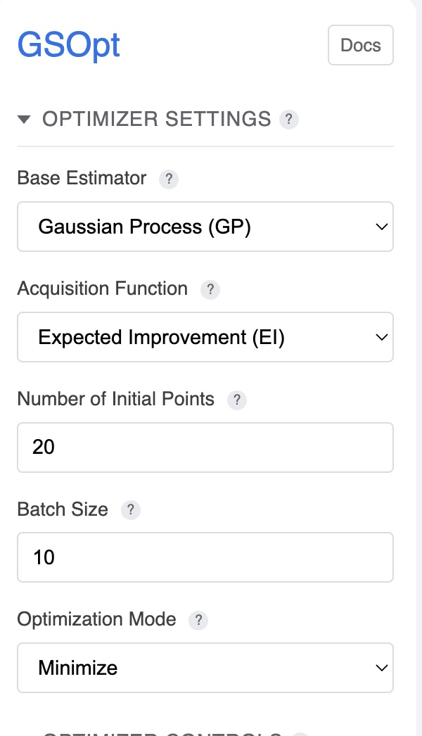
The sidebar provides controls for configuring the optimization algorithm:

• Base Estimator (Regressor): Choose the surrogate model (GP, RF, ET, or GBRT). See The Optimizer section for details.
• Acquisition Function: Select the strategy for choosing new points (gp_hedge, LCB, EI, or PI).
• Kappa (LCB only): Controls the exploration/exploitation trade-off; higher values encourage exploration.
• Optimization Mode: Choose Minimize or Maximize. Maximize will be handled by negating objective values before sending to the backend.
• Batch Size: Number of new points to request per iteration.
• Initial Points: Number of random points sampled before starting model-based optimization.

For recommendations on which settings to use, see Recommendations and Examples.

Optimizer Controls

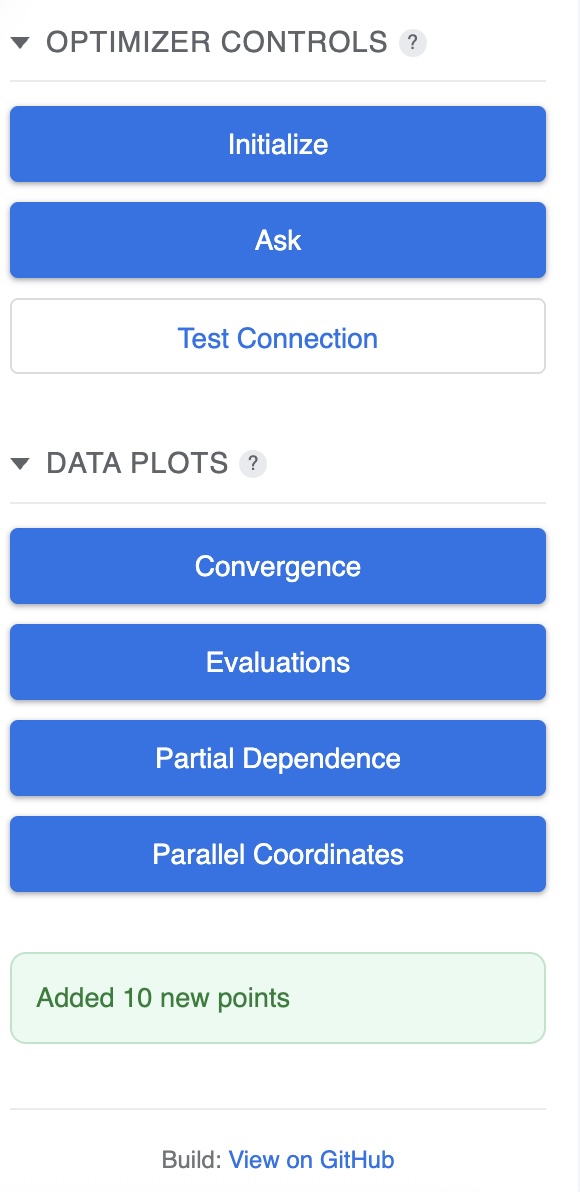
Use the sidebar buttons to control the optimization process:

• Initialize: Generates the initial batch of random points to begin optimization.
• Ask: Requests a new batch of points from the optimizer based on previous results.
• Test Connection: Verifies that the Cloud Run backend is reachable and you have permission.
• Data Plots: Opens advanced visualization dialogs (Convergence, Evaluations, Objective Partial Dependence, Parallel Coordinates).

Entering Data After Initialization

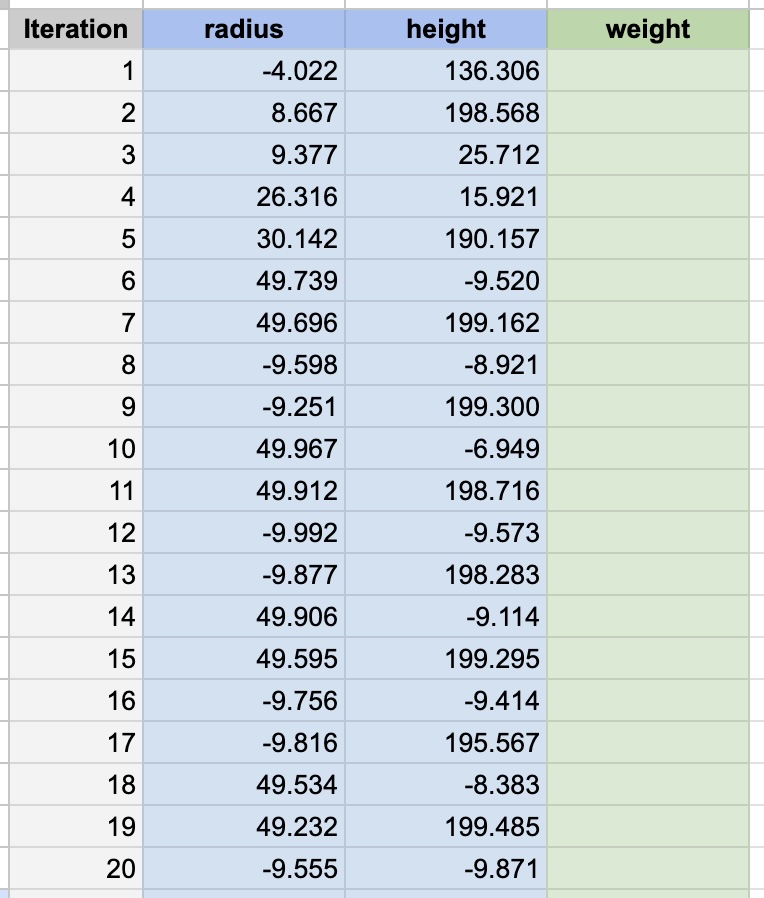
After clicking Initialize, the optimizer will populate the Data sheet with initial parameter combinations to test. Enter the results in the Objective column after running your experiments. In-sheet charts on the Analysis tab will update automatically.

Entering Data After Ask

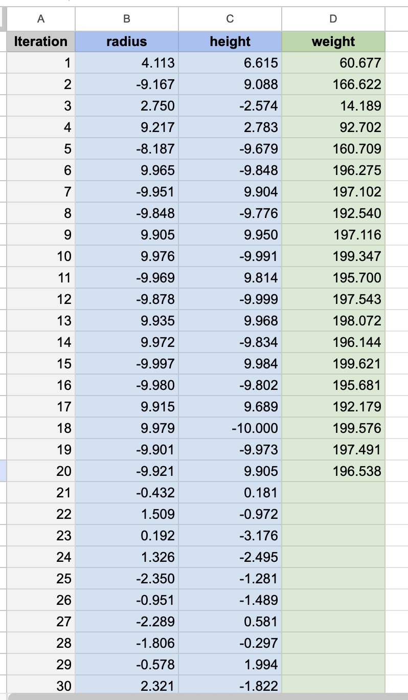
After clicking Ask, new parameter combinations will be added to the Data sheet. Run your experiments and enter the objective values. Repeat the Ask → Experiment → Enter Data cycle to continue optimization.

Convergence Plot

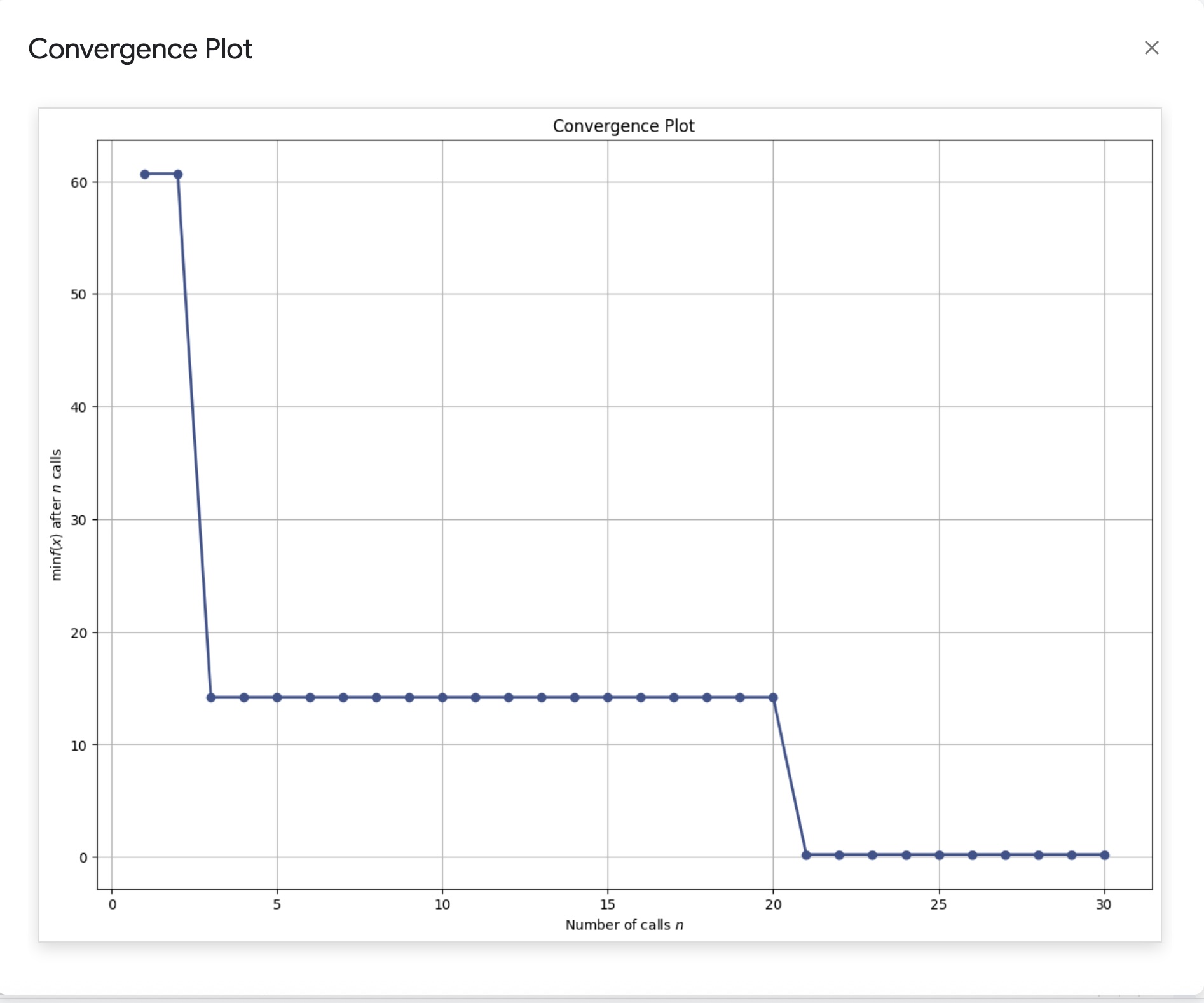
Shows the best objective value found over iterations. For minimization problems, it should generally decrease as better solutions are found.

Evaluations Matrix

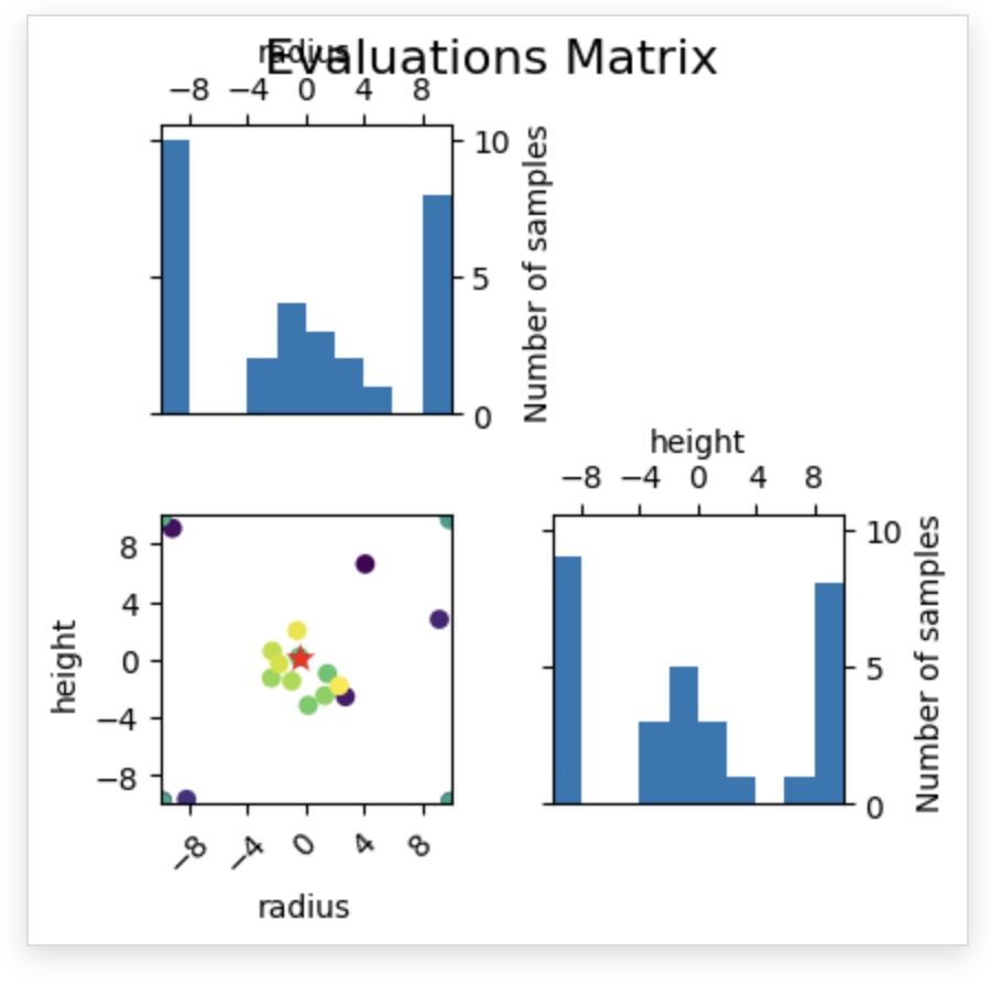
Visualizes sampling locations in parameter space. Over time, you should see clustering around promising regions.

Objective Partial Dependence

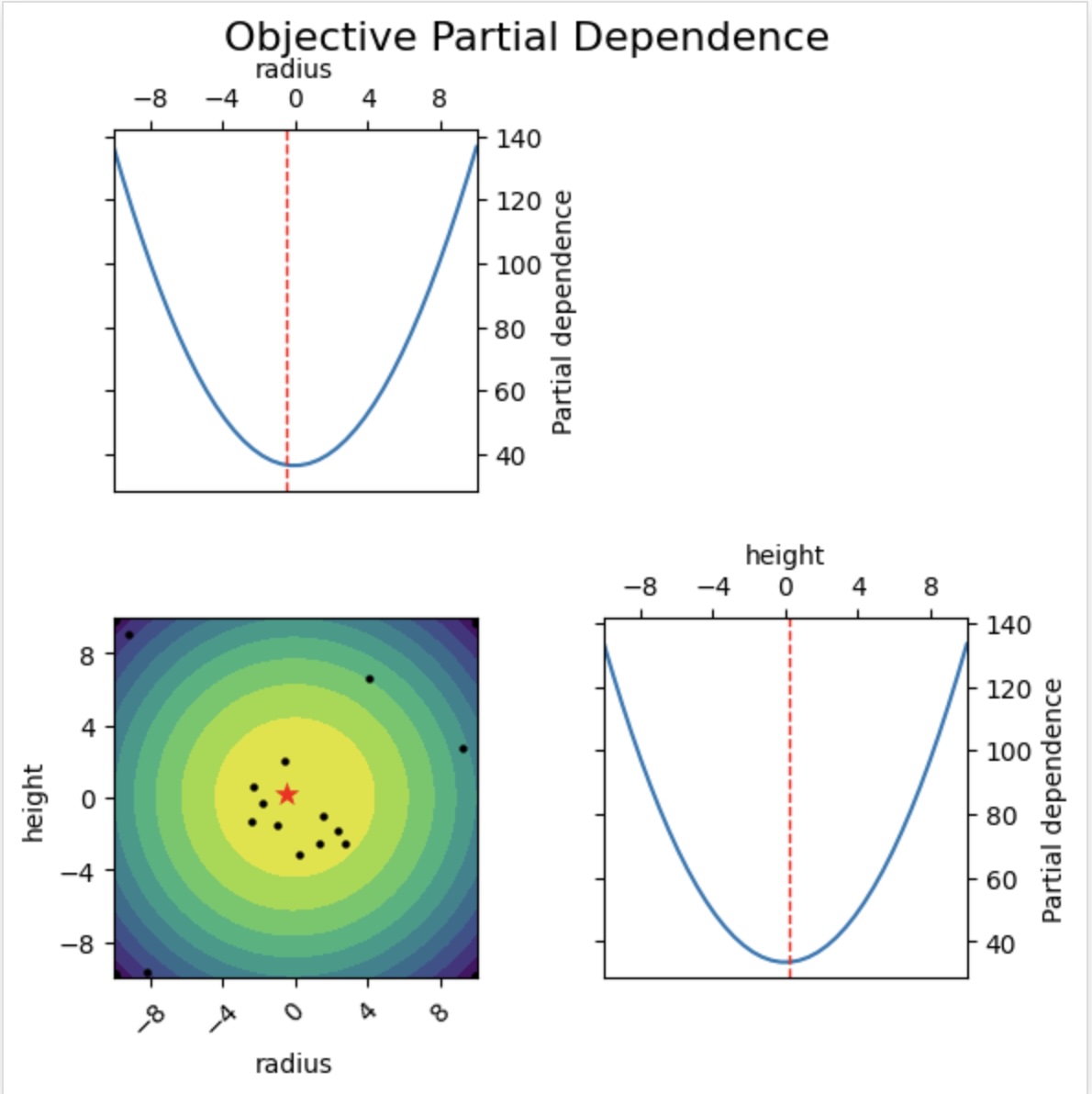
Shows how the modeled objective varies with each parameter while marginalizing over the others. See the scikit-optimize documentation.

Parallel Coordinate Plots

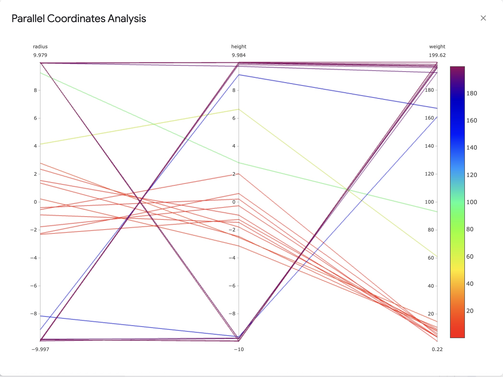
Provides a multi-axis view of parameters and objective values.

Parameter Settings

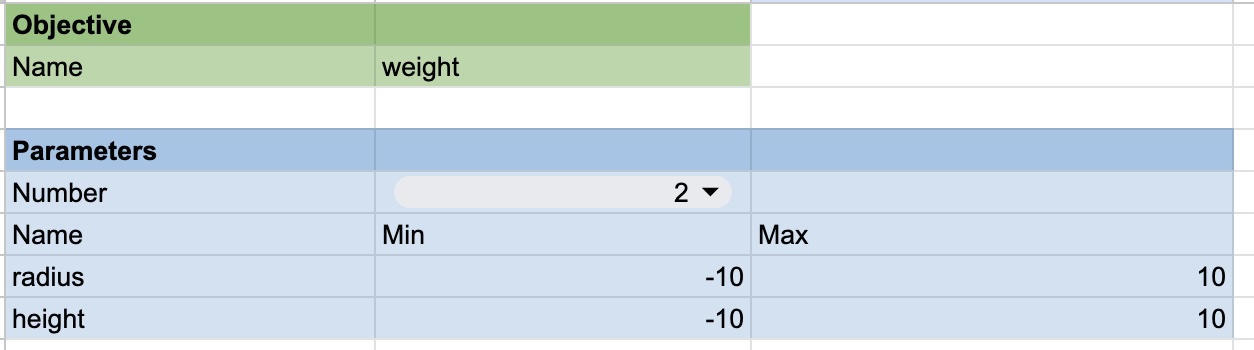
Configure your optimization problem:

• Parameter Names: Provide meaningful names.
• Lower/Upper Bounds: Define the search range for each parameter.
• Objective Name: Sets the label used in headers and plots.

When you update names or the objective in Parameter Settings, headers in the Data sheet update automatically. Charts in the Analysis tab refresh when objective values are edited.

Backend Architecture

The gs-opt backend is a lightweight Python web service built with Flask. It’s designed to be stateless, which makes it robust and easy to deploy on serverless platforms like Google Cloud Run. For each API call, the optimizer is rebuilt from the settings and data provided in the request.

The key components are:

• gsopt.py: The main Flask application that exposes the API endpoints (/init-optimization, /continue-optimization). It handles incoming requests, authenticates the user, and orchestrates the optimization process.
• skopt_bayes.py: A wrapper around the scikit-optimize library that provides a simple “ask” and “tell” interface. The ask method requests new points, and the tell method updates the optimizer with new results.
• utils.py: Contains helper functions for logging and request authentication.

The Optimizer

The optimization is powered by scikit-optimize, a robust and popular library for sequential model-based optimization. gs-opt uses its Bayesian optimizer to intelligently navigate the search space. You can find more details about the library on the scikit-optimize website.

Bayesian Optimization with scikit-optimize

Bayesian optimization is an efficient strategy for finding the maximum or minimum of black-box functions. It works by building a probabilistic model of the objective function (the “surrogate model”) and using that model to select the most promising points to evaluate next. This approach is effective for problems where each function evaluation is costly (e.g., time-consuming experiments or expensive computations).

In gs-opt, you can configure the scikit-optimize backend by choosing the surrogate model (regressor) and the acquisition function.

• Regressor: This is the probabilistic model used to approximate the objective function. While Gaussian Processes are the most common choice for Bayesian optimization, scikit-optimize also supports other tree-based models which can be effective.
  • GP (Gaussian Process): A powerful and common choice for Bayesian optimization due to its ability to provide smooth interpolations and reliable uncertainty estimates for its predictions. This is the recommended default.
  • RF (Random Forest): An ensemble of decision trees. It can capture complex, non-linear relationships but provides a less smooth approximation of the objective function.
  • ET (Extra Trees): Similar to a Random Forest, but with more randomness in how splits in the trees are chosen. This can sometimes help in exploring the search space more effectively.
  • GBRT (Gradient Boosted Regression Trees): An ensemble method that builds trees sequentially, where each new tree attempts to correct the errors of the previous ones. It can be a very powerful model but is sometimes prone to overfitting.
• Acquisition Function: This function guides the search for the optimum. It uses the surrogate model’s predictions and uncertainty estimates to determine the “utility” of evaluating any given point. It balances exploration (sampling in areas of high uncertainty to improve the model) and exploitation (sampling in areas likely to yield a good objective value). The main options available are:
  • gp_hedge: A dynamic strategy that adaptively chooses between several acquisition functions at each iteration.
  • LCB (Lower Confidence Bound): Explicitly balances exploration and exploitation using a parameter kappa. A low kappa favors exploitation, while a high kappa encourages more exploration.
  • EI (Expected Improvement): A classic choice that focuses on the expected amount of improvement over the current best-found value.
  • PI (Probability of Improvement): Similar to EI, but focuses only on the probability of improving over the current best, rather than the magnitude.

Pros and Cons

Pros:

• Sample Efficiency: Bayesian optimization is designed to find good solutions in a minimal number of function evaluations, making it ideal for expensive problems.
• Flexibility: scikit-optimize provides robust and well-tested implementations of various models and acquisition functions.
• Handles Noise: The probabilistic nature of a Gaussian Process surrogate model naturally handles noisy objective functions.

Cons:

• “Curse of Dimensionality”: Performance can degrade as the number of parameters in the search space increases. Always try to minimize the number of dimensions in your optimization.
• Computational Cost: The cost of fitting the surrogate model grows with the number of observations. For this project, this cost is generally negligible compared to the cost of evaluating the objective function itself.

Recommendations and Examples

Based on our testing, we have the following recommendations for starting your optimization:

• General Purpose: For a robust, all-around strategy, we recommend using a Gaussian Process regressor (GP) with the gp_hedge acquisition function. This method dynamically selects the best acquisition function at each step and generally performs well across a variety of problems.

• More Exploitative: If you believe you are close to an optimum and want to focus on refining the solution, we recommend using LCB (Lower Confidence Bound) with a small kappa (e.g., 0.5). This encourages the optimizer to sample in regions it already knows are good.

• More Explorative: If the optimizer seems stuck in a local minimum, or you want to search the parameter space more broadly, we recommend using LCB with a large kappa (e.g., 4.0 or higher). This pushes the optimizer to explore uncertain regions.

Benchmark Test Results

The plots below show the performance of different optimizer configurations on standard benchmark functions. These tests were run using the evaluate.py script in the repository.

Test Configuration

The results were generated with the following settings to simulate a realistic use case:

• Dimensions: 5 (N_DIMS = 5)
• Noise: A small amount of Gaussian noise (NOISE_LEVEL = 0.01) was added to the objective function to simulate real-world measurement error.
• Initial Points: 20 randomly sampled points were evaluated before starting model-based optimization (NUM_INIT_POINTS = N_DIMS * 4).
• Batch Size: 5 new points were requested from the optimizer at each iteration (BATCH_SIZE = N_DIMS).
• Averaging: Each test was run 5 times (NUM_RUNS = 5), and the results were averaged to ensure the conclusions are robust.

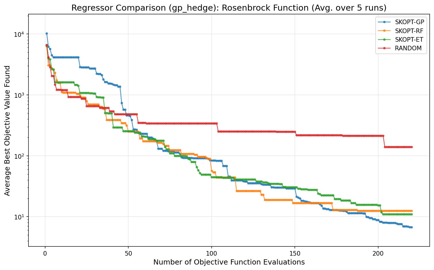
Regressor Performance

The following plot compares the performance of different surrogate models (regressors) on the Rosenbrock function, a classic difficult non-convex problem. All optimizers used the gp_hedge acquisition function. The SKOPT-GP (Gaussian Process) model consistently finds a better solution faster than the tree-based methods.

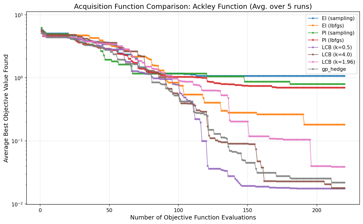
Acquisition Function Performance

This plot compares different acquisition functions for the SKOPT-GP optimizer on the Ackley function, which has many local minima. The gp_hedge strategy shows strong, consistent performance. LCB with a high kappa (k=4.0) is also effective at exploring, while LCB with a low kappa (k=0.5) exploits more and converges slower on this particular problem.

---

Legal

• Privacy Policy
• Terms of Service